Excel Tips - Index Function
The INDEX function in Excel is a powerful lookup function that returns a value at any determined position in an array.
Index Function in Excel
The INDEX function in Excel is a powerful lookup function that returns a value at any determined position in an array. The function can return individual values or entire rows and columns. The INDEX function is typically used in combination with the MATCH function, where the MATCH function sends a position to the INDEX function.
The INDEX function syntax is as follows:
=INDEX (array, row_num, [col_num], [area_num])
array – a range of cells
row_num – the row position in the reference or array
col_num – [this argument is optional] the column position in the reference or array
area_num – [this argument is optional] the range in a reference that will be used
Index Match Function
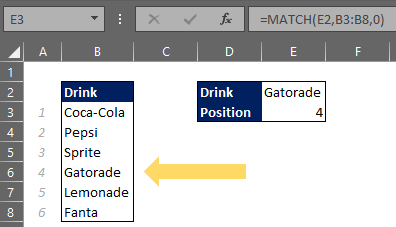
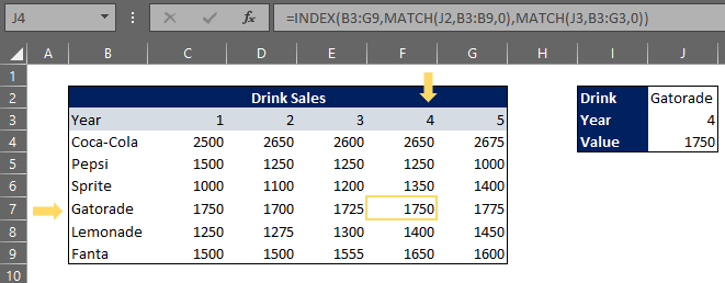
The INDEX function combined with the MATCH function is an even more effective tool. This allows the formula to be dynamic rather than static. The MATCH function imbedded inside of the INDEX function allows users to perform advanced lookups. The MATCH function is used to return any position in an array, whether the array is vertical or horizontal. The MATCH function imbedded inside of the INDEX function can allow flexibility to return positions for either the column or row.
The MATCH function syntax is as follows:
=MATCH (lookup_value, lookup_array, [match_type])
lookup_value – the value that will be matched in the array
lookup_array – the range of cells or an array
match_type – [this argument is optional] 1 is exact or next smallest, 0 is an exact match, -1 is exact or next to largest
Although match type is optional, it is very useful in finding accurate results. If one decides to omit the match type, the automatic default is 1.
1 – In order to find the exact or next smallest value, the array must be sorted in ascending order.
0 – The lookup_array does not need to be sorted in order to find an exact match.
-1 – In order to find the exact match or next largest value, the array must be sorted in descending order.


