Excel Tips for Private Equity: Conditional Formatting

View fullsize

Identifying and analyzing trends or results from large data set calculations can be challenging. With Conditional Formatting in Excel, we can format cells to better illustrate the story the data is trying to tell us.

What is Conditional Formatting?

Conditional Formatting is a feature in Excel that allows you to apply special formatting to cells that meet certain criteria. Typically, conditional formatting is used to color specific cells in order to emphasize or differentiate between values within the spreadsheet. Whether these values are certain investment return requirements, minimums on inventory levels, or cash flow levels, conditional formatting serves to organize data in a more digestible fashion. 

When is it used?

Identifying and analyzing trends or results from large data set calculations can be challenging. It’s hard to see the picture that our data is painting when bogged down in the granular details. In many cases, you may find that visualization can lead to better data interpretation. With Conditional Formatting in Excel, we can format cells to better illustrate the story the data is trying to tell us.

There is an endless number of scenarios where conditional formatting can be useful, it simply depends on the scenario and information you are trying to convey. Nonetheless, conditional formatting has common preset formatting settings that can be helpful for a variety of cases.

How is it used in Real Estate?

At Top Shelf Models, we prefer to use conditional formatting to quickly communicate results in complex models. By using the toggles incorporated into our models, we leverage conditional formatting to “grey out” the cells that are not in use.

For example, we use conditional formatting in our models with mezzanine financing or distribution waterfall calculations to grey out associated cells when they are not in use, thus allowing us to better focus our attention on the values in play. When mezzanine financing or waterfall calculations are needed, we can simply change our toggle and the cells will fill with the associated values.

Additionally, you can use conditional formatting for certain returns and IRR requirements by setting color scales as green for returns above a threshold and as red for returns below. We also incorporate conditional formatting color scales into our sensitivity tables.

---

Presets of Conditional Formatting in Excel

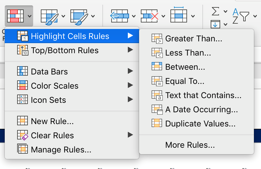
First, conditional formatting allows you to apply highlight rules to your data. Highlight rules are conditions that, if satisfied, highlight the cell are certain color (i.e. green if above a certain $ amount and red if below). You can create highlight rules for a large number of conditions such as “Text that contains ___”, “Duplicate Values”, and “Greater than…” just to name a few.

Next, we have Top/Bottom rules, which allows you to emphasize the bottom or top range of cells based on certain conditions. You can set this formatting for a range of cells based on criteria such as top 10%, bottom 10%, above average, etc.

In addition, data bars and color scales are other preset conditional formatting features which allow you to illustrate your data with a visual bar or color scale. In each case, the length of the bar or the color of the bar represents the value of the cell compared to the other cells in the formatting range.

Finally, Conditional Formatting also provides us with icon sets. We can set certain icons or indicators to call attention to values within the data. Additionally, you can set custom rules under the “New Rule” tab. These custom rules can be written to identify values in the data related to the specific goals of your project and can be a combination of the preset rules or functions within Excel.

---

Example using Multifamily Development Models

In this example, we will be looking at conditional formatting in a simple error check for one of our multifamily development models. Looking at our error check calculations, we immediately see that we are returning icons, so this must be an icon conditional formatting.

When we dive into cell C9, we see that our formula is rounding the difference between Model Output X9 and Monthly CF F41, in this case these are both the annual Effective Gross income. By taking the difference between the same number displayed on different sheets, we ensure that accurate values are displayed throughout the model

When we click on the “Manage Rules” tab of conditional formatting, we pull up all the formats for this sheet. Thus, we can see that our formatting returns a green checkmark if it satisfies the conditions, and a red “X” if it does not. This allows for quick comprehension when looking through our error check.

---

About the Author

Eric Bergin is the founder of TSM. He realized that there was a need for real estate financial models that were more than just generic templates. He wanted to create a personalized product for his customers that would ensure success for them and their company. Please reach out to him if you have any questions on conditional formatting or if he can help you with your modeling needs.